Beta distribution and Dirichlet distribution
July 10, 2021 7 min read
Beta distribution and Dirichlet distribution are Bayesian conjugate priors to Bernoulli/binomial and categorical/multinomial distributions respectively. They are closely related to gamma-function and Gamma-distribution, so I decided to cover them next to other gamma-related distributions.
Beta distribution
In previous posts we’ve already run into Beta-function, an interesting function, closely related to Gamma-function.
While cumulative density function of gamma-distribution is essentially the ratio of partial Gamma-function to a complete Gamma-function, cumulative density function of Beta-distribution is very similar to it - it is just a ratio of incomplete Beta-function to a complete one.
To understand the motivation for Beta distribution, let us consider a common baseball example, popularized by some blogs posts and cross-validated stackexchange answer.
Motivation: moneyball
Beta distribution and Dirichlet distribution are commonly used for pseudo-counts.
Imagine that a new draft class just entered NBA (ok, I admit, I kind of promised you a baseball analogy, but I’m more of a basketball guy, so we’ll go on with 3-pointers, rather than batting averages), and with a limited amount of data available after the first 10 games, you are trying to predict the 3pt percentage of the rookies.
Suppose that throughout the first 10 games a rookie called S. Curry shot 50 3-pointers and hit 22 of them. His 3pt percentage is 44%.
Now, we can be pretty sure he can’t be shooting 44% throughout his whole career, this ridiculous percentage is a result of adrenaline of the first games. So, what you are going to do in order to project his career averages is take the league averages (they are around 37% these days) and mix them with your real observations in some proportion.
Instead of = , where are successes and are total attempts, you’ll going to use . To get a better understanding of conjugate priors, let us move to the next section.
Beta-distribution is a conjugate prior to Bernoulli/binomial
Conjugate priors trivia
Conjugate priors are a (somewhat pseudo-scientific) tool, commonly used in Bayesian inference.
In bayesian statistics you consider both observation and distribution parameter as random variables.
Suppose, you are tossing a coin in a series of Bernoulli trials. The probability of heads is considered a random variable, not just a parameter of distribution. So, the probability of having observed heads in trials using a fair coin is a joint probability distribution.
Now, we know one-dimensional conditional distribution (essentially, all the vertical slices of our joint distribution): if we get fixed, we get a binomial distribution . How can we infer the joint probability distribution?
The answer is, there is no unique way. You cannot observe conditional distributions of one dimension and uniquely identify the other dimension’s conditional (or even marginal) distribution, let alone the joint distribution.
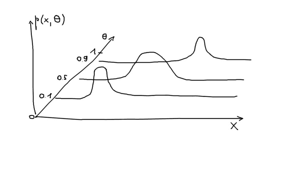
For instance, consider the following 2-dimensional distribution over and :
For this example I assumed that conditional distribution of is binomial with large enough number of trials, so that it converges to normal. Let us fix the value of . Integral of over obviously results in 1. So, to get the marginal distribution over we have to… think it out. There is no single answer. For different marginal (= prior) distributions of we will obtain different joint distributions .
So what Bayesians decided to do instead is to require that posterior and prior distributions of belonged to the same distribution family. Translating this to the multivariate distributions language, conjugate priors ensure that conditional (the vertical slices of our joint probability distribution) and marginal distributions of are consistent, i.e. belong to the same family.
While the choice of conjugate prior as a prior distribution of the parameter is convenient, it is convenient and nothing more - it is completely theoretically unjustified otherwise. For one thing, it does not follow from the shape of conditional distribution . With conjugate priors I would make sure to understand very clearly, what you are “buying”, and not getting oversold on them, before you go out to zealously march in the ranks of Bayesian church neophytes, waving it on your banner.
I have a feeling, that conjugate priors are somewhat similar to copula functions in frequentist (*cough-cough*, even JetBrains IDE spellchecker questions existence of such a word) statistics. Given marginal distributions of two or more random variables, you can recover their joint distribution by assuming a specific dependence between those variables, and this assumption is contained in the choice of a copula function. In case of conjugate priors.
Proof of the fact that Beta distribution is a conjugate prior to binomial
Again, I’ll be following the general logic of another blog post by Aerin Kim with this proof.
Let us show that posterior distribution of indeed belongs to the same family as prior:
.
Dirichlet distribution
Dirichlet distribution to Beta distribution is what multinomial distribution is to binomial.
Dirichlet distribution found multiple applications in (mostly Bayesian) machine learning. One of the most popular approaches to topic modelling, popularized in the early 2000s by Micheal Jordan, Andrew Ng and David Blei, is called Latent Dirichlet Allocation. From the name you could guess that Dirichlet distribution is in its core. It is a subject of a separate post.
References
- http://varianceexplained.org/statistics/beta_distribution_and_baseball/ - moneyball post
- https://stats.stackexchange.com/questions/47771/what-is-the-intuition-behind-beta-distribution/47782#47782 - same moneyball post in the shape of stackoverflow post
- https://www.thehoopsgeek.com/best-three-point-shooters-nba/ - live diagram of NBA all time 3pt percentages and shots made
- https://towardsdatascience.com/conjugate-prior-explained-75957dc80bfb - post on conjugate priors by Aerin Kim

Written by Boris Burkov who lives in Moscow, Russia, loves to take part in development of cutting-edge technologies, reflects on how the world works and admires the giants of the past. You can follow me in Telegram

