Intro to compressed sensing

Motivation: Nyquist-Shannon (Kotelnikov) theorem

Suppose that you have a WAV file. It basically contains sound pressures, measured 44 100 or 48 000 times a second.

Why 44 100/48 000?

Suppose that you want to recover harmonics of frequencies 1 Hz, 2 Hz, 3 Hz, … up to 20 kHz (more or less the upper threshold of what a human ear can hear). Each harmonic of your sound of frequency $\omega_i$ is described by 2 variables: amplitude $A_i$ and phase $\phi_i$.

So, if you are trying to recover those 20 000 pairs of phases/amplitude, you need at least 40 000 of sound pressure measurements $p_i$ measured at moments of time $t_i$, when you apply Fourier transform to recover it. Here it is:

$\begin{cases}A_1 e^{ -\frac{2 \pi j \cdot \omega_1 \cdot (t_1 + \phi_1)}{40000} } + A_2 e^{-\frac{2 \pi j \cdot \omega_2 \cdot (t_1 + \phi_2)}{40000}} + ... + A_{20000} e^{-\frac{2 \pi j \cdot \omega_{20000} \cdot (t_1 + \phi_{20000})}{40000}} = p_1 \\ A_1 e^{ -\frac{2 \pi j \cdot \omega_1 \cdot (t_2 + \phi_1)}{40000} } + A_2 e^{-\frac{2 \pi j \cdot \omega_2 \cdot (t_2 + \phi_2)}{40000}} + ... + A_{20000} e^{-\frac{2 \pi j \cdot \omega_{20000} \cdot (t_2 + \phi_{20000})}{40000}} = p_2 \\ ... \\ A_1 e^{ -\frac{2 \pi j \cdot \omega_1 \cdot (t_{40000} + \phi_1)}{40000} } + A_2 e^{-\frac{2 \pi j \cdot \omega_2 \cdot (t_{40000} + \phi_2)}{40000}} + ... + A_{20000} e^{-\frac{2 \pi j \cdot \omega_{20000} \cdot (t_{20000} + \phi_{20000})}{40000}} = p_{40000} \end{cases}$

Basically, what Nyquist-Shannon theorem states is that there is no way to recover 40000 variables without at least 40000 linear equations.

Or is it?

Compressed sensing

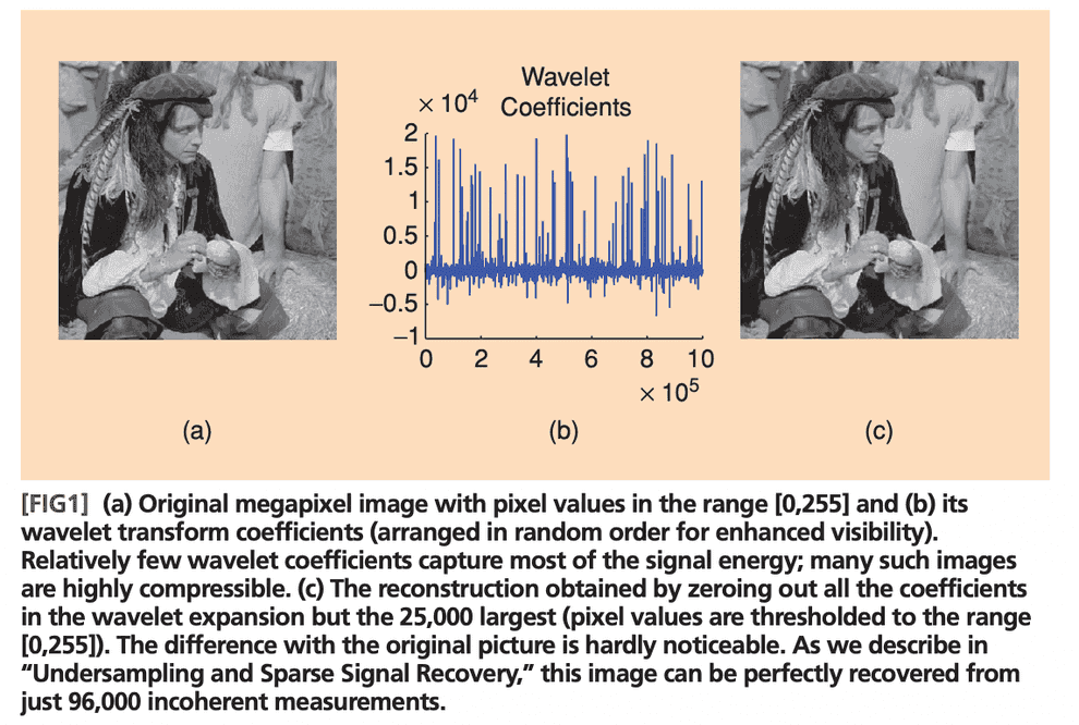
In 1995 Chen and Donoho realised that in reality most of your signals are sparse in some basis. I.e. if you have a recording of music, in reality most of your harmonics have 0 amplitude, and only a very small subset of those are non-zero.

The problem of recovery of $n$ non-zero harmonics out of $N$ is generally NP-hard (this problem can be posed as a constrained optimization of L0 norm).

In 1980s it became clear, however, that you could relax this problem with L0 constraint to a convex problem with L1 constraint, which is still able to recover a small subset of non-zero coefficients, but does this in a small polynomial time.

Chen and Donoho applied this approach to photo compression problems with wavelet transform and achieved spectacular results, even achieving lossless compression.

This approach was popularized 1 year later in the field of statistics by Tibshirani and Hastie, and is now known as Lasso regression or regression with L1 regularization.

The compressed sensing problem could be formulated as follows: you are given a vector of $n$ measurements $\bf y \in \mathbb{R}^n$ (e.g. $n=100$). Those measurement were performed by applying a sensing matrix $A$ to a high-dimensional vector $\bf x \in \mathbb{R}^n$ in $N$-dimensional space, where e.g. $N=40000$.

The trick is that you know that out of the coordinates of $\bf x$ only a small subset is non-zero. The matrix $A$ is $n$-by-$N$, i.e. very wide and very thin. Now, using the Lasso magic you can try to recover your true vector $\bf x$ by approximating it with a vector $\bf \bar{x}$, being a solution of the following convex optimization problem:

$\begin{cases} \min \limits_{\bar{ {\bf x} }} ||\bar{ {\bf x} }||_1 \\ {\bf y} = A {\bf \bar{x}} \end{cases}$

What’s left unclear is how to construct such a sensing matrix and in which basis our signal is expected to be sparse?

Here comes the method of random projections. In an older post I wrote about an incredibly beautiful and unbelievably powerful statement, called Johnson-Lindenstrauss lemma, which basically states that if you project any point cloud of finite amount of points (e.g. ~1000) of arbitrarily large dimensionality $N$ with e.g. gaussian random projection matrix onto a space of small dimensionality $n$ (in the ballpark of ~100-200 dimensions), all the distances between every pair of points will be preserved up to a tiny error with a probability, approaching 1.

Turns out, we can use this gaussian random projection basis (or other basis, satisfying some criteria) as a sensing basis for our signal, and we should be able to recover the full signal of e.g. 40000 harmonics with just a few hundred measurements, if that signal is sparse.

Theorem 1 (exact recovery of sparse signal in noiseless case is bounded by mutual coherence)

In reality our measurement devices are never perfect, and they generate some level of noise, and later on I will show that even noisy measurements allow for compressed sensing.

But first let us consider a “spherical horse in vacuum”, the perfect noiseless measurements case.

We understand now that we can do with $n$ measurements, which is much, much less than $N$, but how big should $n$ be, precisely?

Turns out that $n \ge Const \cdot \mu^2(A) \cdot S \cdot log N$ is enough.

Here:

• $n$ is the number of measurements required
• $N$ is the size of our ambient space
• $S$ is the maximum number of non-zero coordinates in the vector $\bf x$ we strive to recover (this number is called sparcity)
• $A$ is our sensing matrix
• $\mu(A) = \max \limits_{k, j} |A_{k, j}|$ is a bit tricky: it is a quantity, called incoherence

I’ll explain incoherence below.

Signal incoherence

To understand why signal incoherence is important let us consider a perfectly bad sensing matrix: let each row of our matrix be a Dirac’s delta, i.e. every measurement measures just a single coordinate of our data vector. How many measurements will it take to recover all the vector coordinates more or less reliably?

This is a coupon collector’s problem: on average $N \cdot \log N$ measurements will be required to measure every single one of $N$ coordinates of our data vector.

In this case our sensing matrix is called perfectly coherent: all the “mass” of our measurement is concentrated in a single coordinate. Incoherent measurements matrices, on the other hand, are those that have their mass spread evenly. Note that we impose a condition that $l2$ norm of each vector of the sensing matrices is limited down to $\sqrt{N}$.

Examples of incoherent and coherent sensing matrices

• Dirac’s delta - poor sensing matrix, coherent, see coupon collector problem
• Bernoulli random matrix - an incoherent sensing matrix
• Gaussian random matrix - another incoherent sensing matrix
• (possibly incomplete) Fourier Transform matrix - even better sensing matrix
• random convolution - good sensing matrix (incoherence can be seen in Fourier domain)

See lecture by Emmanuel Candes.

Sensing matrix as a product of measurement matrix and sparsity inducing matrix

In practice sensing matrix $A$ is a bit constrained.

First, its rows are supposed to have an L2 norm of $\sqrt{N}$. With this constraint $\mu(A)$ varies in range 1 to $\sqrt{N}$. If the “mass” is evenly spread between rows of $A$, the matrix is incoherent and is great for compressed sensing. If all the “mass” is concentrated in 1 value, the matrix is highly coherent, and we cannot get any advantage from compressed sensing.

Second, the sensing matrix of measurements cannot be arbitrary, it is determined by the physical nature of measurement process. Typical implementation of the measurement matrix is a Fourier transform matrix.

Third, our initial basis might not be the one, where the signal is sparse.

Hence, we might want to decompose our matrix $A$ into a product of two matrices: measurement matrix and sparsity basis matrix: $A = \Phi \Psi$.

For instance, consider one vertical line of an image. The image itself is not sparse. However, if we applied a wavelet transform to it, in the wavelet basis it does become sparse. Hence, $\Psi$ matrix is the matrix of wavelet transform. Now, $\Phi$ is the measurement matrix: e.g. if you have a digital camera with a CMOS array or some kind of a photofilm, the measurement matrix $\Phi$ might be something like a Fourier transform.

Now we can give a new interpretation to our signal incoherence requirement:

$\mu(A) = \max \limits_{k, j} | \langle \phi_k, \psi_j \rangle |$

This means that every measurement vector (e.g. Fourier transform vector) should be “spread out” in the sparsity-inducing basis, otherwise the compressed sensing magic won’t work. For instance, if l2-norm of our sensing matrix vectors is fixed to be $\sqrt{N}$, if all the vector values are 0, and one value is $\sqrt{N}$, the sensing magic won’t work, as all the “mass” is concentrated in one point. However, if it is spread evenly (e.g. all the coordinates of each vector have an absolute value of 1), that should work perfectly, and the required number of measurements $n$ would be minimal.

Theorem 1: exact formulation and proof outline

The exact formulation of Theorem 1 is probabilistic: set a small enough probability $\delta$, e.g. $\delta=0.001$.

Then with probability not less than $\delta$ the exact recovery of $S$-sparse vector $\bf x$ with a sensing matrix $A$ is exact, if the number of measurements $n \ge C \cdot S \cdot \mu^2(A) \cdot (\log N - \log \delta)$.

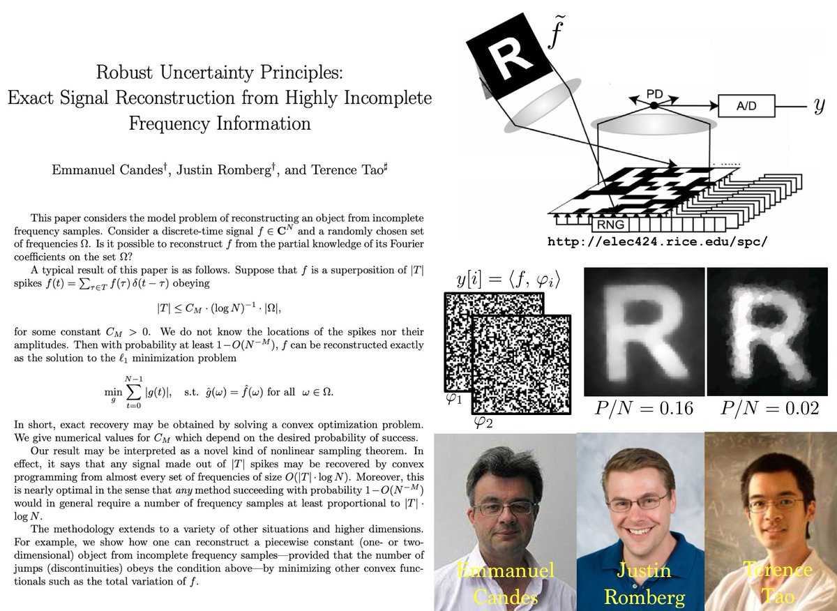
There are multiple proofs by Candes and Tao (an initial proof, specialized for partial Fourier transform as sensing matrix, its extension for arbitrary unitary sensing matrices and, finally, a simplified proof in Lecture 4 of the series of Cambridge lectures by Emmanuel Candes).

Step 1: dual certificate guarantees uniqueness of the solution

To prove this step I am following lecture 2 by E.Candes and a separate paper with a good proof.

Dual norm to the vector norm $||x||$ is $|| y ||_d = \max \limits_{|| x || \le 1} \langle y, x \rangle$.

Lemma 1.1. Dual problem to the constrained norm minimization problem

Given a minimization problem $\min || x ||$, constrained on $Ax = b$, the corresponding dual problem to it is:

$\max \limits_{\alpha} \langle \alpha, b \rangle$, constrained on $|| \alpha^T A ||_d \le 1$

To see this consider the Lagrangian:

$\mathcal{L}(x, \alpha) = || x || + \alpha^T (b - Ax)$

$\mathcal{L}(x, \alpha) = ||x||(1 - \alpha^T A \frac{x}{||x||}) + \alpha^T b$

Now, minimize this Lagrangian. Expression $\alpha^T A \frac{x}{||x||}$ is actually used in the dual norm: $u = \frac{x}{||x||}$ is a vector with norm 1.

Hence, $x^* = \arg \min \limits_x \mathcal{L}(x, \alpha) = \arg \max \limits_{x} \alpha^T A u = || \alpha^T A ||_d$.

Now we see, that if $|| \alpha^T A ||_d \le 1$, the Lagrangian attains its minimum at: $\mathcal{L}^* = \alpha^T b$, when $||x|| \to 0$.

If $|| \alpha^T A ||_d > 1$, Lagrangian can be made arbitrarily small by increasing $||x|| \to \infty$.

Lemma 1.2. Lasso dual problem

Observe that the norm, dual to L1 is L-infinity:

$|| \alpha ||_\infty = \max \limits_{||x||_1 = 1} \langle \alpha, x \rangle$

Thus, by Lemma 1.1, Lasso dual problem is:

$\max \limits_{\alpha} \alpha^T b$, given $|| \alpha^T A ||_\infty \le 1$.

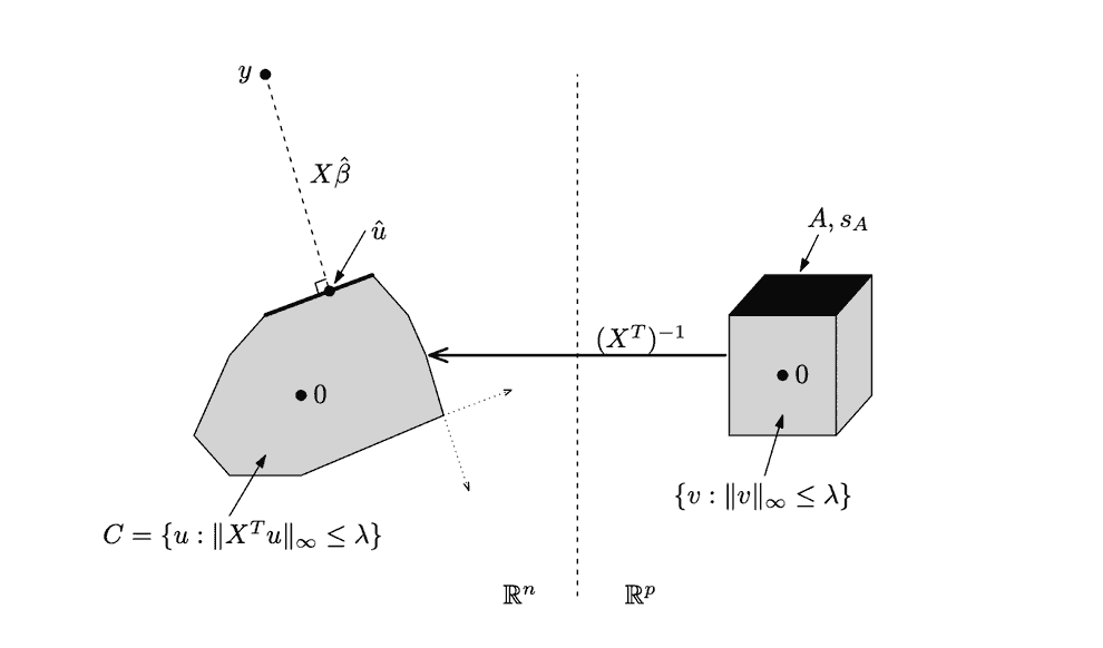
Here is a graphical interpretation of the dual problem by Ryan Tibshirani

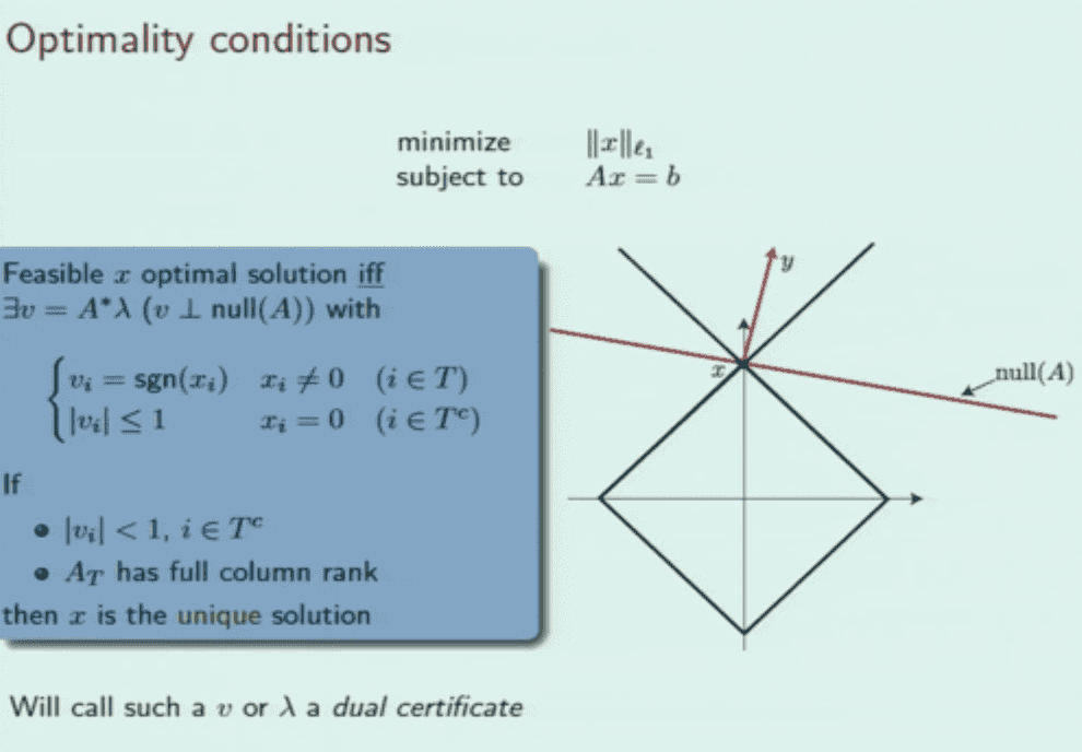
Lemma 1.3. For any feasible vector x, its dual equals the sign of x for non-zero coordinates x[i]

$\alpha^T A [i] = \text{sign}(x [i])$ if $x[i] \neq 0$

Applying strong duality, we get:

$||x||_1 = \alpha^T b = \alpha^T A x = \sum_i \alpha^T A[i] x[i]$

Hence, $\alpha^T A [i] = \text{sign}(x [i])$ (otherwise, some components will cancel each other out and we’ll achieve the value of L1 norm less than $||x||_1$, given that $|| \alpha^T A ||_\infty \le 1$).

Lemma 1.4. Uniqueness of dual certificate

I am following E.Candes lecture 2 here.

Suppose that we’ve managed to find a solution to our primal problem $\bar{x}$.

Let us prove that any other feasible solution $x_1$ is worse than $\bar{x}$. Denote $S$ the set of indices $i$, where $\bar{x}[i]$ is non-zero. Denote $S_c$ the complementary set of indices $i$, where $\bar{x}[i] = 0$.

Denote $h = \bar{x} - x$ the vector of difference between $\bar{x}$ and $x$. Obviously, $h$ lies in the null space of operator $A$, so that if $A\bar{x} = y$, $Ax = y$ as well. Thus, $Ah = y$, too.

Denote $v = \begin{cases} \text{sign}(\bar{x}[i]), \text{if } i \in S \\ v_i, \text{where} |v_i| \le 1, \text{if } i \in S_c \end{cases}$ the dual certificate vector.

Now, suppose there is another vector $x$, which has a smaller L1 norm than our solution $\bar{x}$. Let us show, that this is impossible.

Consider L1 norm of $x$:

$||x||_1 = ||\bar{x} + h||_1 = || \bar{x} + h_S ||_1 + || h_{S_c} ||_1 \ge || \bar{x} ||_1 + \sum \limits_{i \in S} \text{sign}(\bar{x})[i]h_S[i] + || h_{S_c} ||_1$

Now, note that $\sum \limits_{i \in S} \text{sign}(\bar{x})[i]h_S[i]$ is part of our dual certificate here:

$|| \bar{x} ||_1 + \sum \limits_{i \in S} \text{sign}(\bar{x})[i]h_S[i] + || h_{S_c} ||_1 = || \bar{x} ||_1 + \sum \limits_{i \in S} v_i h_i + || h_{S_c} ||_1 \ge$

$\ge || \bar{x} ||_1 + \langle v, h \rangle + \sum \limits_{i \in S_c}(1 - |v_i|) || h ||_1$

Now recall that our dual certificate is orthogonal to the null space of $A$, i.e. $\langle v, h \rangle = 0$. Hence:

$||x||_1 \ge || \bar{x} ||_1 + \sum \limits_{i \in S_c} (1 - |v_i|) || h ||_1$

As the absolute value of each coordinate of the dual certificate on $S_c$ set is smaller than 1, we just guaranteed that $||x||_1 \ge ||\bar{x}||_1$, unless $x = \bar{x}$.

Step 2: a way to construct a dual certificate

I am following this tutorial on compressed sensing.

Now we show that with overwhelming probability it is possible to construct the dual certificate.

$v = A^T A_S (A_S^T A_S)^{-1} sign(\bar{x})_S$ and also $v^T = \alpha^T A$, hence, $\alpha = A_S (A_S^T A_S)^{-1}sign(\bar{x})_S$.

Let us write SVD of $A^S = U S V^T$. Then $A_S^T A_S = V S U^T U S V^T = V S^2 V^T$, then $(A_S^T A_S)^{-1} = V^{-T} S^{-2} V^{-1}$.

Then $A_S (A_S^T A_S)^{-1} = U S V^T V^{-T} S^{-2} V^{-1} = U S^{-1} V^{-1}$, and recalling that $V$ is orthogonal, $V^{-1} = V^T$, $A_S (A_S^T A_S)^{-1} = U S^{-1} V^{-1} = U S^{-1} V^T$.

Now suppose that the diagonal matrix of non-negative singular values $S$ has largest signular value $\sigma_1$ and smallest singular value $\sigma_S$. Hence, the largest singular value of $S^{-1}$ is $\frac{1}{\sigma_S}$.

This allows us to have an upper limit the L2 norm of our vector $\alpha$:

$||\alpha||_2 = || U S^{-1} V^T sign(\bar{x})_S ||_2 \le \frac{||sign(\bar{x})_S||_2}{\sigma_S} = \frac{\sqrt{S}}{\sigma_S}$

Now, recall that $v^T = \alpha^T A$ or $v = A^T \alpha$.

Consider each coordinate of the vector $v_i = A_i^T \alpha$. Random variables $\frac{A_i^T \alpha}{||\alpha||_2^2}$ are standard Gaussian random variables, hence, for them holds the following simple inequality:

$p(|\xi| \ge t) \le 2 e^{\frac{-t^2}{2}}$

Applying this inequality, we get:

$p(| A_i^T \alpha | \ge 1) = p(\frac{| A_i^T \alpha|}{|| \alpha ||_2} \ge \frac{1}{||\alpha||_2}) \le 2e^{-\frac{1}{2 ||\alpha||^2_2}} = 2e^{-\frac{\sigma_S^2}{2S}}$

Now, due to inequalities, such as Johnson-Lindenstrauss lemma, we can obtain limits on largest and smallest singular values of our matrix A_S: $\sigma_S \ge 0.5 \sqrt{n}$, where $n$ is the number of measurements in compressed sensing.

Hence $p(|| A_i^T \alpha || \ge 1) \le 2 e^{-\frac{n}{8S}}$.

Now we want to limit the probability that $v_i \ge 1$ for all $i \in S^c$ of our vector $v$.

Thus, we get $p (\forall v_i \le 1) = 1 - (1 - p(|| A_i^T \alpha || \ge 1))^N \le N p(|| A_i^T \alpha || \ge 1) \le N e^{-\frac{n}{8S}}$

and $n \ge C \cdot S \cdot \log p (\forall v_i \le 1) \cdot \log N$

We now see how the required number of measurements $n$ depends on total dimensionality $N$ and sparsity $S$, and we can choose it so that $\log p (\forall v_i \le 1)$ can be made arbitrarily small, and dual certificate is almost guaranteed to exist in practice.

Step 3 (optional): operator Bernstein inequality

I am following the appendix of this paper on matrix completion

Alternatively, one can use operator versions of exponentiated Markov inequalities.

Recall that $A^T$ is a random matrix and apply operator form of Bernstein inequality (I will outline its proof in the next step) to the operator norm $|| A^T ||$ or to a random vector $|| A^T \alpha ||$.

Operator form of Bernstein inequality is a stronger form of Bernstein inequality for random variables, which is, in turn, a strong alternative version of Markov inequality (a.k.a. Chebyshev’s first inequality in Russian tradition).

Recall Markov (a.k.a. Chebyshev’s first) inequality:

$p(\xi \ge \epsilon) \le \frac{\mathbb{E} \xi}{\epsilon}$

If we potentiate both sides of inequality inside the probability term, a number of useful inequalities follow, such as Chernoff bound, Hoeffding inequality and Bernstein inequality. Specifically, Bernstein inequality for a sum of independent random variables states that:

$p(|\frac{1}{n} \sum \limits_{i=1}^n \xi_i| \ge \epsilon) \le e^{- \frac{n \epsilon^2}{2 (1 + \frac{\epsilon}{3})}}$

Now, instead of random variables $\xi_i$ consider random matrices $A_i$. Replace absolute value with spectral norm:

$p(||\frac{1}{n} \sum \limits_{i=1}^n A_i|| \ge \epsilon) \le e^{- \frac{n \epsilon^2}{2 (1 + \frac{\epsilon}{3})}}$

The proof can be seen here. It makes use of an operator version of Markov (Chebyshev’s first) inequality, operator Chernoff bound, Golden-Thompson inequality and, finally, operator Bernstein inequality.

Speaking informally, matrices $A_{\Omega T}$ are almost orthogonal with overwhelming probability. Take note of this fact, it will be central for Theorems 2 and 3 in deterministic approach.

Robustness of compressed sensing

For compressed sensing to be applicable to real-life problems, the technique should be resistant to corruptions of the data. They are of two kinds:

• First, in reality the vectors $x$ in the sensing basis might not be exactly $S$-sparse, there might be some noise.
• Second, the obtained measurements $y_i$ in reality are likely to be corrupted by some noise as well.

Amazingly, compressed sensing is resistant to both of these problems, which is provable by theorems 2 and 3 respectively.

Restricted isometry property (RIP) and its flavours

While theorem 1 has a probabilistic nature, even more powerful theorems 2 and 3 have deterministic nature. To pose them we’ll need another property, called restricted isometry.

Recall that a crucial part of the proof of Theorem 1 was the fact that $A_{\Omega T}^* A_{\Omega T}$ matrix was almost orthogonal. A similar requirement is made even stronger with Restricted Isometry Property (RIP).

For some constant, reflecting the sparsity of vector $x_S$, $\delta_S < 1$ any sub-matrix $A_{\Omega T}$ of matrix $A$:

$(1 - \delta_S) || x ||_2 \le || A_{\Omega T} x ||_2 \le (1 + \delta_S) || x ||_2$

In plain english this means that if $A$ is a rectangular “wide” $n \times N$ matrix, and $x_S$ is a sparse vector with all of its $N$ coordinates zero, except by a subset of coordinates $T$ of cardianality $|T| = S$, any sub-matrix $A_{\Omega T}$ with all rows removed, but those in $T$, is almost orthogonal and preserves the lengths of vectors $x$ it acts upon, up to a constant $\delta_S$. Almost-orthogonality of matrix $A_{\Omega T}$ follows from length preservation because $|| x ||_2 = x^T x = x^T A_{\Omega T}^T A_{\Omega T} x$.

In my opinion, even more useful form of an equivalent statement is distance preservation:

$(1 - \delta_S) || x_1 - x_2 ||_2 \le || A_{\Omega T} (x_1 - x_2) ||_2 \le (1 + \delta_S) || x_1 - x_2 ||_2$

If this requirement seems contrived to you, consider several practical examples of matrices, for which RIP holds.

Random Gaussian matrix: Johnson-Lindenstrauss lemma and random projections

Consider a $n \times N$ matrix, of which each element is a realization of a random normal variable. These matrices are used for random projections.

For such matrices a super-useful Johnson-Lindenstrauss lemma is known, which states that with overwhelmingly high probability such matrices preserve distances between points and lengths of vectors.

Obviously any sub-matrix of a random Gaussian matrix is itself a random Gaussian matrix, so Johnson-Lindenstrauss lemma allows for a probabilistic version of RIP to hold, if we use random Gaussian projections as our sensing matrix.

Random Bernoulli/binary matrix: Kashin-Garnaev-Gluskin lemma

A similar case are random binary matrices: each element of such a matrix is a Bernoulli random variable, taking values of $\{1, -1\}$.

TODO: Kolmogorov width and Gelfand width

TODO: Kashin-Garnaev-Gluskin lemma

Partial Fourier transform matrix: Rudelson-Vershinin lemma

A similar result was proven by Mark Rudelson and Roman Vershinin for partial Fourier transform matrices.

TODO: mention $\log^5$ convergence

Theorem 2 (robust recovery of a sparse subset of the largest vector coordinates, even if the vector is not sparse)

Suppose that in reality our vector $\bf x$ is not $S$-sparse, but is corrupted with perturbations. Let us denote its S-sparse sub-vector with only S non-zero coordinates $\bf x_S$.

E.g. ${\bf x} = \begin{pmatrix} 0.1 \\ 1 \\ 2 \\ 0.2 \end{pmatrix}$ and ${\bf x_S} = \begin{pmatrix} 0 \\ 1 \\ 2 \\ 0 \end{pmatrix}$ being $S=2$-sparse.

Then:

$||{\bf \bar{x}} - {\bf x}||_1 \le C_S \cdot || {\bf x} - {\bf x_S} ||_1$ and $|| {\bf \bar{x}} - {\bf x}||_2 \le C_S \cdot \frac{ || {\bf x} - {\bf x_S} ||_1}{\sqrt{S}}$

In plain english, l2 norm of the difference between the sparse vector $\bf \bar{x}$, recovered by compressed sensing, and $S$-sparse subset of vector $\bf x$ is no greater than l2 norm of the remainder of $\bf x$, after we subtract the vector $X_S$ which contains the $S$ largest in absolute value coordinates from it.

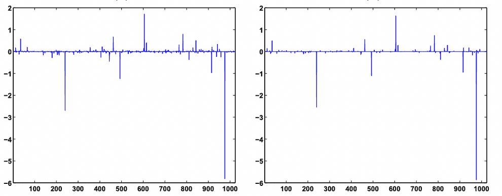
Here is an example of reconstruction of an approximately (but not perfectly) sparse signal by compressed sensing. Note that some low-amplitude noise is discarded by compressed sensing, resulting in a slightly sparser signal, than it was originally:

TODO: tightness of compressed sensing by Kashin-Garnaev-Gluskin lemma

Theorem 3 (robust recovery of sparse signal upon noisy measurements)

Now that “things got real”, let us make them even more real: our measurement process is imperfect, too. Assume that we have some noise in measurements, but it is bounded in l2 norm with a parameter $\epsilon$. Hence, we are solving the following problem now:

$\begin{cases} \min || {\bf \bar{x}} ||_1 \\ || A {\bf \bar{x}} - {\bf y} ||_2 \le \epsilon \end{cases}$

Theorem 3 states that this problem can be solved efficiently, too:

$|| {\bf \bar{x}} - {\bf x} ||_2 \le \underbrace{C_0 \cdot \epsilon}_\text{measurement noise} + \underbrace{C_1 \cdot \frac{|| {\bf x} - {\bf x_S} ||_1}{\sqrt{S}}}_\text{noise in sparsity of recovered vector}$

Putting this simply, the l2 error in recovery of the sparse signal is limited by a weighted sum of two errors: noise of measurement and non-exact sparseness of the input vector. If both of them are not too large, the recovery can be quite accurate.

Theorem 3 and Theorem 2 proof outlines

I am following two papers: a short one by E.Candes and a long one by the whole team.

Theorem 2 proof

We need to show that in the noiseless case (i.e. for any feasible $x$, $Ax = y$):

$||x-\bar{x}||_1 \le С ||\bar{x}_{S^c}||_1$

Or, denoting $h = x-\bar{x}$:

$||h||_1 \le С ||\bar{x}_{S^c}||_1$

Lemma 2.1. L1 cube/cone constraint

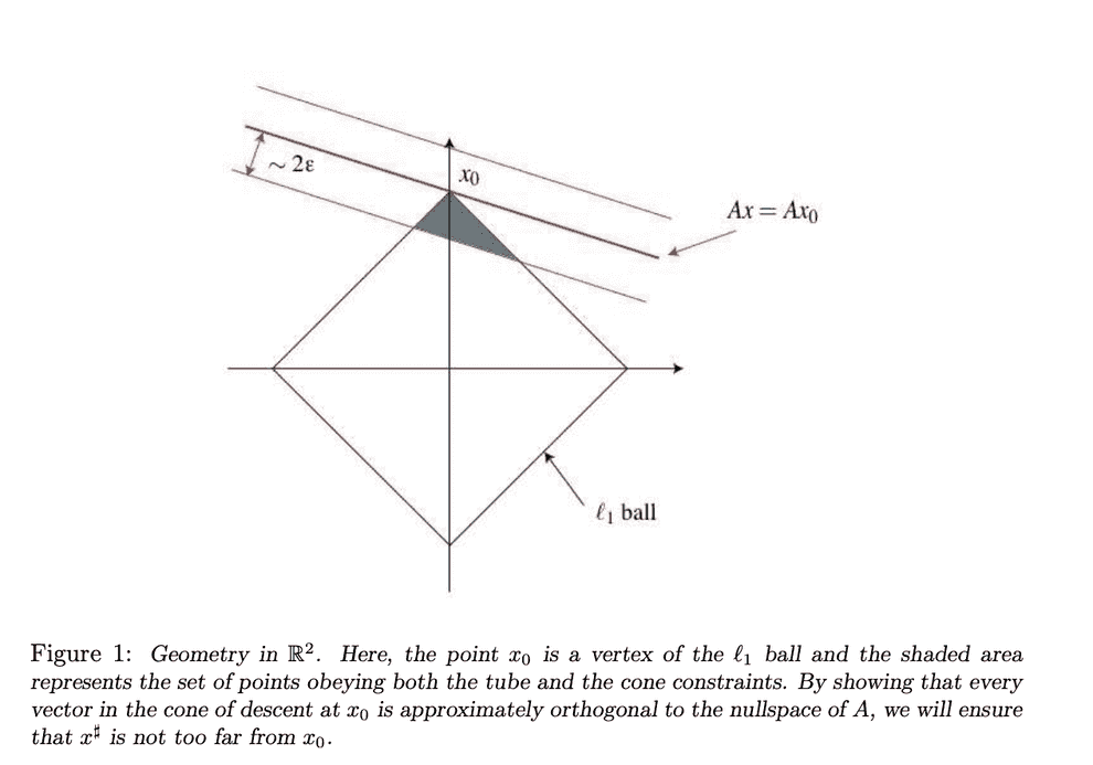
First step to construct this inequality is the cone constraint:

$||\bar{x}||_1 = ||\bar{x}_S||_1 + ||\bar{x}_{S_c}|| \ge ||\bar{x} + h||_1 = ||x_{S_0} + h_{S_0}||_1 + ||x_{S_c} + h_{S_c}|| \ge$

$\ge ||\bar{x}_S||_1 - ||h_{S}||_1 - ||\bar{x}_{S_c}||_1 + ||h_{S_c}||_1$

$||\bar{x}_S||_1 + ||\bar{x}_{S_c}||_1 \ge ||x_{true_S}||_1 - ||h_{S}||_1 - ||\bar{x}_{S_c}||_1 + ||h_{S_c}||_1$

$||h_{S}||_1 \ge ||h_{S_c}||_1 - 2 ||\bar{x}_{S_c}||_1$

or $||h_{S_c}||_1 - ||h_{S}||_1 \le 2 ||\bar{x}_{S_c}||_1$

This is very close to what we need. If we could find a way to express $||h_{S}||_1$ and $||h_{S_c}||_1$ through $||h||_1$ - we’d be done.

Lemma 2.2. RIP application

Here the RIP comes in handy:

$0 = ||Ah||_2 = ||A (h_{S} + \sum \limits_{j=1} h_{S_j})||_2 \ge ||A h_{S}||_2 - ||\sum \limits_{j=1} A h_{S}||_2 \ge ||A h_{S_0}||_2 - \sum \limits_{j=1} ||A h_{S_j}||_2 \ge$

$\ge (1-\delta_{|S|})||h_{S}||_2 - (1+\delta_{|S_j|}) \sum \limits_{j=1} ||h_{S_j}||_2$.

Equivalently, $(1-\delta_S) ||h_{S}||_2 \le (1+\delta_{|S_j|}) \sum \limits_{j=1} ||h_{S_j}||_2$.

Now what’s left is to convert these L2 norms to L1 norm. Luckily, we have:

Lemma 2.3. L2 norm bounds L1 from both top and bottom

$||x||_2 \le ||x||_1 \le \sqrt{\dim x} ||x||_2$

Left part of the inequality holds due to Pythagoras theorem, right part - due to Cauchy-Schwarz inequality.

$\sum \limits_j ||h_{S_j}||_2 \le \sqrt{|S_j|} \sum \limits_j || h_{S_j} ||_{\infty} \le \frac{1}{\sqrt{|S_j|}} \sum \limits_j ||h_{S_{j-1}}||_1$

Applying this to where we left, we get:

$\frac{(1-\delta_S)||h_S||_1 }{\sqrt{S}} \le (1-\delta_S) ||h_{S}||_2 \le (1+\delta_{|S_j|}) \sum \limits_{j=1} ||h_{S_j}||_2 \le (1+\delta_{|S_j|}) \sum \limits_{j=1} ||h_{S_j}||_1 = (1+\delta_{|S_j|}) ||h_{S_c}||_1$

Hence, $\frac{(1-\delta_S)}{\sqrt{S} (1+\delta_{S_c})} ||h_S||_1 \le ||h_{S_c}||_1$

Identially, $||h||_1 = ||h_S||_1 + ||h_{S_c}||_1 \ge ||h_{S}||_1 (1 + \frac{(1-\delta_S)}{\sqrt{S} (1+\delta_{S_c})})$

Or, $||h_{S}||_1 \le \frac{1}{(1 + \frac{(1-\delta_S)}{\sqrt{S} (1+\delta_{S_c})})} ||h||_1$

Substituting this back to $||h_{S_c}||_1 - ||h_{S}||_1 = ||h||_1 - 2 ||h_{S}||_1 \le 2 ||\bar{x}_{S_c}||_1$, we get:

$2 ||\bar{x}_{S_c}||_1 \ge ||h||_1 - 2 ||h_S||_1 \ge ( 1 - 2 \cdot \frac{1}{(1 + \frac{(1-\delta_S)}{\sqrt{S} (1+\delta_{S_c})})}) ||h||_1$

$||\bar{x}_{S_c}||_1 \ge ( \frac{1}{2} - \frac{1}{(1 + \frac{(1-\delta_S)}{\sqrt{S} (1+\delta_{S_c})})}) ||h||_1$ or $||h||_1 \le C_S ||\bar{x}_{S_c}||_1$.

The theorem also contains a clause $||h||_2 \le C_S \frac{||\bar{x}_{S_c}||_1}{\sqrt{S}}$, which follows the fact that $||h||_2 \le ||h||_1$. Not sure about the exact origins of $\frac{1}{\sqrt{S}}$ multiplier, though.

This concludes the proof.

Theorem 3 proof

We need to show that:

$|| \bar{x} - x ||_2 \le C || \bar{x}_{S_c}||_1 + C_1 \epsilon$

Theorem 3 follows the general logic of Theorem 2, but now our measurements are noisy, so the application of RIP now requires a Tube constraint.

Lemma 3.1.Tube constraint

Suppose that true point $\bar{x}$ resulted in a measurement $y$, but due to noise a different solution $x$ was found. This solution is still going to lie within a tube of radius $\epsilon$, surrounding the null space of $A$:

$|| A (\bar{x} - x) ||_2 = ||(A\bar{x} - y) - (Ax - y)||_2 \le || A \bar{x} - y ||_2 + || A x - y ||_2 \le 2 \epsilon$

Both $\bar{x}$ and $x$ are feasible solutions, resulting in measurement $y$ with some l2 noise.

If we substitute the result of lemma 3.1 into the lemma 2.2, we get:

$\frac{(1-\delta_S)}{\sqrt{S} } ||h_S||_1 \le (1+\delta_{S_c}) ||h_{S_c}||_1 + 2 \epsilon$ or $||h_S||_1 \le \frac{\sqrt{S} \cdot (1+\delta_{S_c})}{1-\delta_S} ||h_{S_c}||_1 + 2 \epsilon \frac{\sqrt{S}}{1-\delta_S}$

Now apply lemma 2.1:

$||h_{S_c}||_1 - ||h_{S}||_1 \le 2 ||\bar{x}_{S_c}||_1$, hence:

$||h_{S_c}||_1 - 2||\bar{x}_{S_c}||_1 \le ||h_{S}||_1 \le \frac{\sqrt{S} \cdot (1+\delta_{S_c})}{1-\delta_S} ||h_{S_c}||_1 + 2 \epsilon \frac{\sqrt{S}}{1-\delta_S}$

$||h_{S_c}||_1 (1 - \frac{\sqrt{S} \cdot (1+\delta_{S_c})}{1-\delta_S}) \le 2||\bar{x}_{S_c}||_1 + 2 \epsilon \frac{\sqrt{S}}{1-\delta_S}$

$||h_{S_c}||_1 (1 - \frac{\sqrt{S} \cdot (1+\delta_{S_c})}{1-\delta_S}) \le 2||\bar{x}_{S_c}||_1 + 2 \epsilon \frac{\sqrt{S}}{1-\delta_S}$ or

$||h_{S_c}||_1 (\frac{\sqrt{S} \cdot (1+\delta_{S_c})}{1-\delta_S} - 1) \ge 2||\bar{x}_{S_c}||_1 + 2 \epsilon \frac{\sqrt{S}}{1-\delta_S}$

Now recall that $2||h_{S_c}||_1 - ||h||_1 \le 2 ||\bar{x}_{S_c} ||_1$ or $||h_{S_c}||_1 \le ||\bar{x}_{S_c} ||_1 - \frac{1}{2} ||h||_1$ and get:

$(\frac{\sqrt{S} \cdot (1+\delta_{S_c})}{1-\delta_S} - 1) (||\bar{x}_{S_c} ||_1 - \frac{1}{2} ||h||_1) \ge ||h_{S_c}||_1 (\frac{\sqrt{S} \cdot (1+\delta_{S_c})}{1-\delta_S} - 1) \ge 2||\bar{x}_{S_c}||_1 + 2 \epsilon \frac{\sqrt{S}}{1-\delta_S}$

$(\frac{\sqrt{S} \cdot (1+\delta_{S_c})}{1-\delta_S} - 3) ||\bar{x}_{S_c} ||_1 - 2 \epsilon \frac{\sqrt{S}}{1-\delta_S} \ge ||h||_1 \cdot \frac{1}{2} \cdot (\frac{\sqrt{S} \cdot (1+\delta_{S_c})}{1-\delta_S} - 1)$

$||h||_1 \cdot \frac{1}{2} \cdot (\frac{\sqrt{S} \cdot (1+\delta_{S_c})}{1-\delta_S} - 1) \le (\frac{\sqrt{S} \cdot (1+\delta_{S_c})}{1-\delta_S} - 3) ||\bar{x}_{S_c} ||_1 - 2 \epsilon \frac{\sqrt{S}}{1-\delta_S}$

$||h||_1 \le C_1 || \bar{x}_{S_c} ||_1 + C_2 \epsilon$

As $||h||_2 \le ||h||_1$, this leads to:

$||h||_2 \le C_1 || \bar{x}_{S_c} ||_1 + C_2 \epsilon$.

Practical example

Let us generate a wav-file with a simple chord:

Let us take a perfect piano and consider a Discrete Cosine Transform of A-E-A chord (I don’t want to deal with complex numbers in this case, otherwise, I’d use Fourier).

I’ll open a Jupyter-notebook and programmatically generate DCT spectrum of this signal, then synthesize an artificial wav-file with sound pressures out of it and play it:

import numpy as np
import matplotlib.pyplot as plt
from scipy import fftpack
from scipy.io import wavfile
from IPython.display import Audio

dim = 48000

a_e_a_chord_dct = np.zeros(dim)

a_e_a_chord_dct[440] = 1
a_e_a_chord_dct[660] = 1
a_e_a_chord_dct[880] = 1


generated_wav = idct(a_e_a_chord_dct)

Audio(generated_wav, rate=dim)

Sounds like a chord, right?

Now, let us show that with compressed sensing we don’t have to measure our sound at 48 000 points a second, we will be able to recover the initial signal pretty accurately from just 100 measurement points.

import random
import math

from sklearn import linear_model


# generate a DCT matrix to select just a few random rows from it and use them as a sensing matrix
I = np.identity(dim)
dct_matrix = dct(I)

n_measurements = 100  # measure the sound pressure at this amount of points 


def get_random_indices(n_indices=n_measurements, dim=dim):
    output = []
    counter = 0
    while counter < n_indices:
        prospective_random_index = math.floor(random.random() * dim)
        if prospective_random_index not in output:
            output.append(prospective_random_index)
            counter += 1
        else:
            pass  # redraw, if random index was already used
    
    return output


# select a few rows from our DCT matrix to use this partial DCT matrix as sensing matrix
random_indices = get_random_indices()
partial_dct = np.take(dct_matrix, get_random_indices(), axis=1)

# measure sound pressures at a small number of points by applying sensing matrix to the signal spectrum
y = np.dot(partial_dct.T, a_e_a_chord_dct)

# make the measurement noisy
noise = 0.01 * np.random.normal(0, 1, n_measurements)
signal = y + noise

# recover the initial spectrum from the measurements with L1-regularized regression (implemented as sklearn's Lasso in this case)
lasso = linear_model.Lasso(alpha=0.1)
lasso.fit(partial_dct.T, signal)
for index, i in enumerate(lasso.coef_):
    if i > 0:
        print(f"index = {index}, coefficient = {i}")

index = 440, coefficient = 0.9322433129902213
index = 660, coefficient = 0.9479368288017439
index = 880, coefficient = 0.9429783262003731

Here we go, using just 100 noisy measurements we’ve managed to perfectly recover the spectrum of our signal, and made just 6-7% error in amplitudes.

Let us listen to the result:

recovered_wav = idct(lasso.coef_)
Audio(recovered_wav, rate=dim)

Can your ear tell the difference? I can not.

Magic!

References

• https://authors.library.caltech.edu/10092/1/CANieeespm08.pdf - a great introduction to compressed sensing by Emmanuel Candes and Michael Wakin
• https://cims.nyu.edu/~cfgranda/pages/MTDS_spring19/notes/duality.pdf - an amazing full paper on Compressed sensing from lagrange duality to Theorem 1
• https://www.youtube.com/watch?v=zytez36XlCU - a good talk on compressed sensing by Richard Baraniuk
• https://asa.scitation.org/doi/10.1121/1.5043089 - another good introduction to compressed sensing
• https://studylib.net/doc/10391762/the-johnson-lindenstrauss-lemma-meets-compressed-sensing-… - an early paper by Richard Baraniuk and Michael Wakin on merging J-L lemma with compressed sensing
• https://personal.utdallas.edu/~m.vidyasagar/Fall-2015/6v80/CS-Notes.pdf - a long and complicated introduction to compressed sensing by Mathukumalli Vidyasagar
• https://www.turpion.org/php/reference.phtml?journal_id=rm&paper_id=5168&volume=74&issue=4&type=ref - results by Boris Kashin
• http://www.mathnet.ru/present12903 - a talk on related topic by Boris Kashin
• https://arxiv.org/pdf/math/0611957.pdf - paper on incoherence Theorem 1 by Candes and Romberg
• https://arxiv.org/pdf/math/0503066.pdf - paper on compressed sensing by Candes, Romberg and Tao
• https://www.eecis.udel.edu/~amer/CISC651/IEEEwavelet.pdf - introduction to wavelets
• https://www.youtube.com/watch?v=y7KLbd7n75g - good introduction to wavelets by Steve Brunton
• https://www.youtube.com/watch?v=ZnmvUCtUAEE - another helpful introduction to wavelets
• https://en.wikipedia.org/wiki/Eigenvalue_perturbation - eigenvalue perturbation
• https://asa.scitation.org/doi/10.1121/1.5043089 - compressed sensing in acoustics
• https://sms.cam.ac.uk/collection/1117766 - lectures by E.Candes in Cambridge (most importantly, see 2, 3, 4)
• https://arxiv.org/pdf/math/0409186.pdf - early paper on special case of Theorem 1
• https://arxiv.org/pdf/math/0410542.pdf - second paper on Theorem 1
• https://arxiv.org/pdf/math/0611957.pdf - more mature paper on Theorem 1
• https://www.sciencedirect.com/science/article/pii/S1631073X08000964 - short proof of theorems 3 and 2
• https://arxiv.org/pdf/math/0503066.pdf - paper on 2 versions of Theorem 3
• https://sprjg.github.io/posts/compressed_sensing_with_the_fourier_ensemble/ - practical example of compressed sensing
• https://piazza.com/class_profile/get_resource/hidzt72ukxiol/hj1e7hcsupf3th - on dual certificates
• https://cims.nyu.edu/~cfgranda/pages/MTDS_spring19/notes/duality.pdf - lemma on dual certificate (and another proof of Theorem 1)
• https://arxiv.org/pdf/0910.0651.pdf - advance paper on matrix completion by Candes co-author Benjamin Recht with a proof of operator Chernoff bound
• https://authors.library.caltech.edu/23952/1/Candes2005.pdf - error correction codes with compressed sensing by Candes, Tao, Vershinin, Rudelson
• https://math.stackexchange.com/questions/701062/derivative-of-the-nuclear-norm/704271#704271 - nuclear norm via semidefinite programming
• https://math.stackexchange.com/questions/746332/dual-of-a-semidefinite-program/746883#746883 - dual of semidefinite programming problems
• https://www.math.cuhk.edu.hk/~lmlui/dct.pdf - explanation of DCT, quantization and sparse coding in JPEG
• https://www.youtube.com/watch?v=DS8N8cFVd-E - video about DCT in JPEG

Written by Boris Burkov who lives in Moscow, Russia, loves to take part in development of cutting-edge technologies, reflects on how the world works and admires the giants of the past. You can follow me in Telegram