Survival analysis - survival function, hazard rate, cumulative hazard rate, hazard ratio, Cox model
June 11, 2021 7 min read
Here I discuss the statistics apparatus, used in survival analysis and durability modelling.
Hazard rate and survival function
“Death of a person is a tragedy, deaths of millions is statistics” - Joseph Stalin
Hazard rate is just a renormalization of the probability space that takes pallid impersonal statistics on input and converts it into your own chances to live another day.
Suppose you’re an average young man in the Wild West. You decide to pursue a questionable career of a train robber.
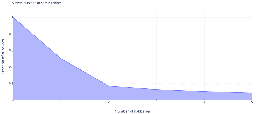
Assume that the chance of an average guy surviving his first train robbery is . After that you get slightly more experienced and for your second train robbery your chance of survival is . Now, you’re even more experienced and for the third stint the chance of survival is .
So the night before your third robbery you might ask yourself, whether it is worth the risk of dying with 25% chance tomorrow, or should you rather give up on train robberies altogether and move on to start a career in finance?
The data you want to ask yourself this question is the chance of survival tomorrow, which is the Hazard rate.
Unfortunately, it’s impossible to get the data about your odds in the real life. What you could do instead is take a look at the cumulative distribution function of a train robber’s life expectancy, or, rather its counterpart , called the survival function:
Probability mass function (which is a discrete-case analogue of the continuous probability density function) of dying at your third robbery . We can more or less reformulate this as a continuous problem , where is a random variable indicating the number of robberies an average train robber survives, , is cumulative distribution function and is probability density function.
So you see, probability density function/probability mass function answers a wrong question. It says that out of all repeat train robbers the fraction that dies at their third robbery is (). But the question you want to ask is: if I go for my third robbery tomorrow, what are my chances to survive it, and the answer you want is .
Now, let’s start formalizing this. For a discrete-time variable, Hazard function is your chance to die during your next robbery number :
Thus, hazard function is defined as:
Or, in continuous-time case:
In a continuous-time case instead of simply potentiating the hazard rate, you need to wrap your head around integrating the hazard function. Let us calculate the risk a person would accumulate over a period of time t by induction:
, thus summing those up:
…
Again, from Bayesian point of view hazard rate (multiplied by ) can be viewed as .
Cumulative hazard rate
The integral of hazard rate that we used in the previous section, is useful in itself.
If it is taken between points of time 0 and t: , it is called cumulative hazard rate .
Cumulative hazard rate is a funny thing. It essentially enumerates and sums up all the chances of death you escaped by the current moment. So, for instance, at your first train robbery you had a chance to die of , at the second - , at the third - .
So by the time you start contemplating your fourth robbery, the “number of deaths” you deserved by now , so in a fair world you would have already been more than dead, exercising your luck so readily…
A corollary from the definition of cumulative hazard rate is its connection to survival function:
, hence, .
Cox proportional hazards model and hazard ratio
Sir David Cox has come up with a linear regression-ish model for factors, influencing the hazard ration:
For Cox proportional hazards models you’d often consider log hazard rate instead of the hazard rate itself.
Hazard ratio reflects the difference in hazards rates for models with different values of factors. For instance for patients 1 and 2 with different values of some factor:
Then the hazard ratio equals:
I can’t say much on this subject as I haven’t used these models yet.

Written by Boris Burkov who lives in Moscow, Russia, loves to take part in development of cutting-edge technologies, reflects on how the world works and admires the giants of the past. You can follow me in Telegram

