Pearson's Chi-square tests - intuition and derivation

In one of my previous posts I derived the chi-square distribution for sum of squares of Gaussian random variables and showed that it is a special case of Gamma distribution and very similar to Erlang distribution. You can look them up for reference.

A motivational example

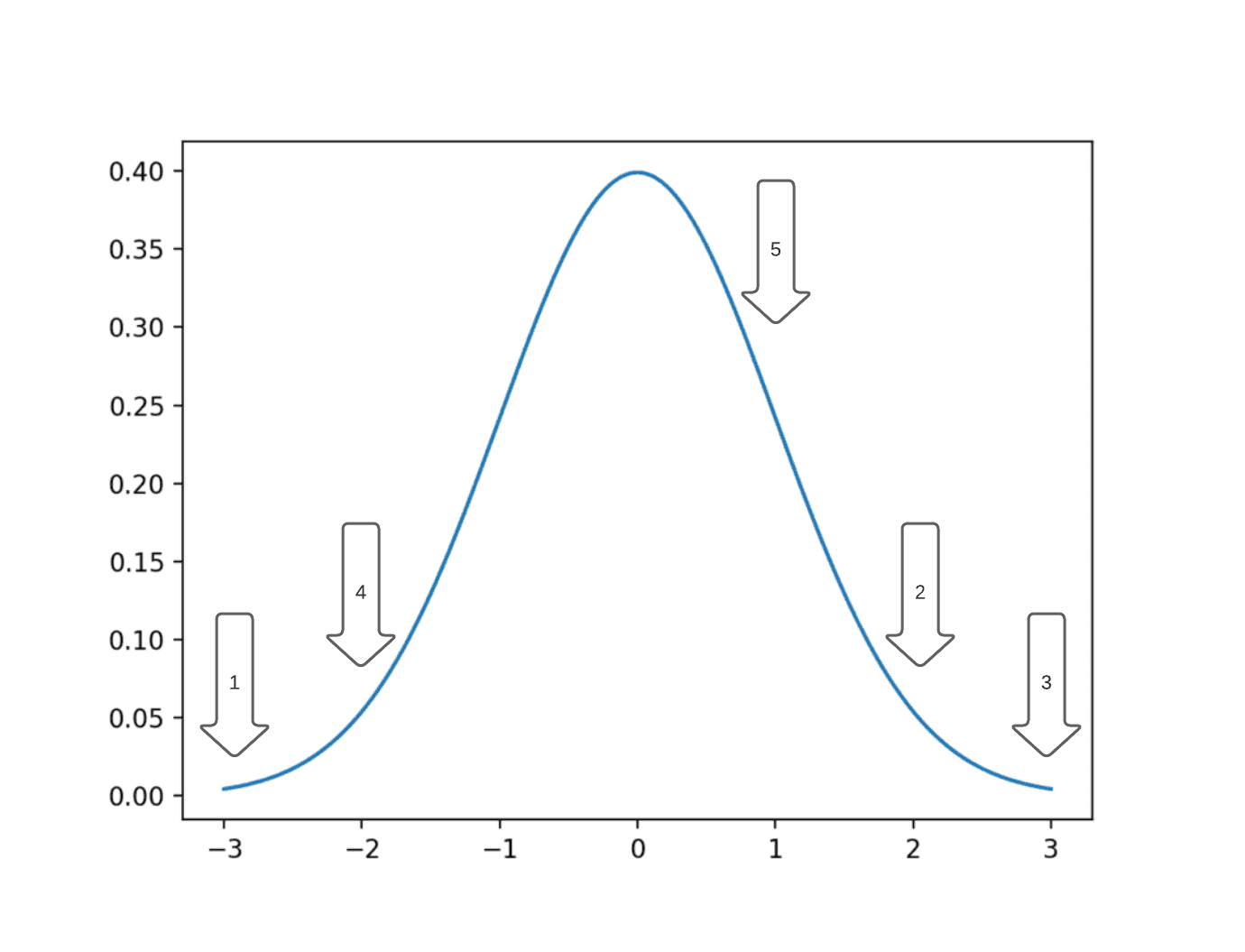
Suppose you’ve taken 5 samples of a random variable that you assumed to be standard normal Gaussian and received suspicious results: you have a feeling that your dots have landed too far away from the peak of distribution.

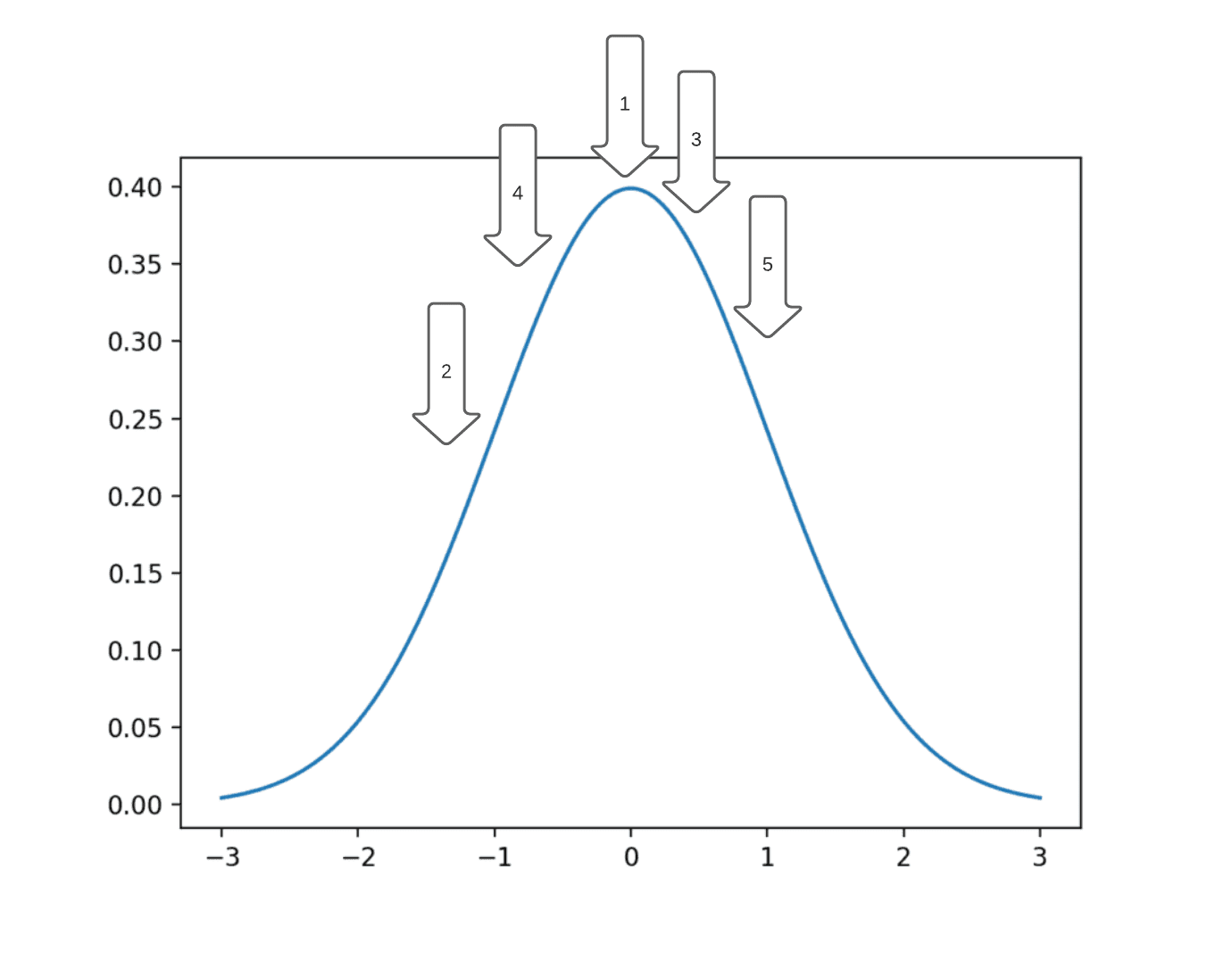
Given the probability density function (abbreviated pdf) of a gaussian distribution and knowledge that standard deviation is 1, you would expect a much more close distribution of your samples, something like this:

You could ask yourself a question: what is the average value of probability density function that I would observe, when sampling a point from standard normal?

Well, you can actually calculate it, following the expectation formula: $\int \limits_{-\infty}^{+\infty} \underbrace{ \frac{1}{\sqrt{2 \pi}} e^{-\frac{x^2}{2}} }_\text{This is the variable you're averaging} \cdot \underbrace{ \frac{1}{\sqrt{2\pi}} e^{-\frac{x^2}{2}}}_\text{This is pdf over which you're averaging} \cdot dx = \frac{1}{ 2\pi } \int \limits_{-\infty}^{+\infty} e^{-x^2} dx$.

Now, substitute $t = \sqrt{2}x$: $\frac{1}{ 2\pi } \int \limits_{-\infty}^{+\infty} e^{-x^2} dx = \frac{1}{ 2\pi } \int \limits_{-\infty}^{+\infty} e^{-\frac{t^2}{2}} d(\frac{t}{\sqrt2}) = \frac{1}{\sqrt{2} \cdot 2\pi } \int \limits_{-\infty}^{+\infty} e^{-\frac{t^2}{2}} dt = \frac{\cancel{\sqrt{2\pi}}}{\sqrt{2}\cdot \sqrt{2\pi} \cancel{\sqrt{2\pi}}} = \frac{1}{\sqrt{2} \sqrt{2\pi}}$.

So, probability density function of an average point, you sample, is expected to be $\frac{1}{\sqrt{2} \sqrt{2 \pi}} = 0.707106 \cdot 0.398942 = 0.282095$.

Let us calculate pdf for several points:

if x=0 (which is the most probable point), your $f_\xi(0)=\frac{1}{ 2\pi } e^{-0/2} = 0.398942$, a bit more probable than average.

if x=1 (which is the standard deviation), your $f_\xi(1)=\frac{1}{ 2\pi } e^{-1/2} = 0.241970$, a bit less probable than average.

if x=2 (which is 2 standard deviations), your $f_\xi(2)=\frac{1}{ 2\pi } e^{-4/2} = 0.053989$, not much.

if x=3 (which is 3 standard deviations), your $f_\xi(3)=\frac{1}{ 2\pi } e^{-9/2} = 0.004432$, very small.

With these numbers let’s return to the 5 points I’ve observed. Out of those five point two points are at 3 standard deviations, two points are at 2 standard deviations and one point is at 1 standard deviation. So the probability density function of such an observation is $f^2_\xi(3) \cdot f^2_\xi(2) \cdot f_\xi(1) = 0.004432^2 \cdot 0.053989^2 \cdot 0.241970 = 1.38 \cdot 10^{-8}$.

At the same time the expected pdf of five average point to be observed is $0.282095^5 = 0.0017863$.

Seems like our observation was a really improbable one, it is less probable than average by over 100 000 times.

Intuition behind Pearson’s chi-square test

We need a more rigorous tool than just comparison of the probability of our observed five points with the average.

Let us call our vector of observations $X = (x_1, x_2, x_3, x_4, x_5)^T$. The combined pdf to observe exactly our 5 points is a 5-dimensional multidimensional standard normal distribution $\frac{1}{\sqrt{2\pi}^5} e^{-\frac{x_1^2 + x_2^2 + x_3^2 + x_4^2 + x_5^2}{2}}$.

But note that we don’t want exactly our point. Any “equiprobable” point will do. For instance, $e^{-\frac{1+1+1+1+1}{2}} = e^{-\frac{0+2+1+1+1}{2}}$, the 5-dimensional points $(1,1,1,1,1)^T$ and $(0,\sqrt{2},1,1,1)^T$ are “equiprobable”, and we want to group them into one.

So, we are actually interested in the distribution of the sum $x_1^2+x_2^2+x_3^2+x_4^2+x_5^2$ as for identical values of the sum the pdfs of likelihood of a vector of observations $X = (x_1, x_2, x_3, x_4, x_5)^T$ are identical.

Each $x_i \sim \mathcal{N}(0, 1)$ is a standard Gaussian-distributed random variable, so the sum in question is a random variable distributed as Chi-square: $\sum \limits_{i}^{N} x_i^2 \sim \chi^2_N$. Please, refer to my older post on Gamma/Erlang/Chi-square distribution for the proof.

That’s why chi-square distribution is the right tool to answer the question, we’re interested in: is it likely, that the observed set of points was sampled from a standard normal distribution.

Derivation of Pearson’s goodness of fit test statistic

The chi-square test is widely used to validate the hypothesis that a number of samples were taken from a multinomial distribution.

Suppose you’ve rolled a $k=6$-sided dice $n=120$ times, and you expect it to be fair. You would expect $E_i=20$ occurrences of each value of the cube $i \in$ {1,2,3,4,5,6} (row E - expected), instead you see some different outcomes $O_i$ (row O - observed):

We need to estimate the likelihood of an outcome like this, if the dice was fair. Turns out that a certain statistic based on these data follows the chi-square distribution: $\chi_{k-1}^2 =\sum \limits_{i}^{k} \frac{(O_i-E_i)^2}{E_i}$. I’ll prove this fact here by induction for increasing number of dice sides $k$ loosely following some constructs from de Moivre-Laplace theorem (which is a special case of Central Limit Theorem, proven before the adoption of much more convenient Fourier analysis techniques).

Induction base: 2-sided dice (coin)

$\sum \limits_{i=1}^{k=2} \frac{(O_i - E_i)^2}{E_i} = \frac{(O_1 - np)^2}{np} + \frac{((n-O_1) - n(1-p))^2}{n(1-p)} = \frac{(O_1-np)^2}{np} + \frac{(O_1-np)^2}{n(1-p)} = \frac{(O_1 -np)^2(1-p) + (O_1 -np)^2p}{np(1-p)} = \frac{(O_1-np)^2}{np(1-p)}$

Now recall that $\xi_1 = \frac{O_1-np}{\sqrt{np(1-p)}} \sim \mathcal{N}(0, 1)$.

Thus, $\xi_1^2 = \frac{(O_1-np)^2}{np(1-p)} \sim \chi^2_1$.

Induction step: (k+1)-sided dice from k-sided dice

In order to perform the induction step, we need to show that if we had a k-dice described by a k-nomial distribution and could apply $\chi_{k-1}$ test to it, there is a way to construct a dice with k+1 sides from it, so that it can be described by a (k+1)-nomial distribution and validated by a $\chi_{k}$ test.

Here’s an example to illustrate the process of creation of an additional side of our dice.

Imagine that we had a continuous random variable, representing the distribution of human heights. We transformed the real-valued random variable of height into a discrete one by dividing all people into one of two bins: “height < 170cm” and “height >= 170cm” with probabilities $p_1$ and $p_2$, so that $p_1+p_2 = 1$. Chi-square test works for our data according to induction basis. We can see sampling of a value from this r.v. as a 2-dice roll (or a coin flip).

Now we decided to split the second bin (“height >= 170cm”) into two separate bins: “170cm <= height < 180cm” and “height >= 180cm”. So, what used to be one side of our 2-dice has become 2 sides, and now we have a 3-dice. Let’s show that Chi-squared test will just get another degree of freedom (it’s going to be $\chi_2^2$ instead of $\chi_1^2$ now), but will still work for our new 3-dice.

Let’s write down the formula of Pearson’s test for 3-nomial disitrubion and split it into binomial part and an additional term:

$\sum \limits_{i=1}^{3} \frac{(O_i - np_i)^2}{np_i} = \frac{(O_1 - np_1)^2}{np_1} + \frac{(O_2 - np_2)^2}{np_2} + \frac{(O_3 - np_3)^2}{np_3} = \underbrace{\frac{(O_1 - np_1)^2}{np_1} + \frac{(O_2 + O_3 - n(p_2 + p_3))^2}{n(p_2 + p_3)}}_{\sum \limits_{j=1}^2 \frac{{O'-np_j}^2}{np_j} \sim \chi_1^2 \text{ for sum of k=2 terms by induction base}} - \underbrace{\frac{(O_2 + O_3 - n(p_2 + p_3))^2}{n(p_2 + p_3)} + \frac{(O_2 - np_2)^2}{np_2} + \frac{(O_3 - np_3)^2}{np_3}}_{\text{this part should also be } \sim \chi_1^2 \text{, let's prove this}}$

Let us focus on the second term and simplify it:

$- \frac{(O_2 + O_3 - n(p_2 + p_3))^2}{n(p_2 + p_3)} + \frac{(O_2 - np_2)^2}{np_2} + \frac{(O_3 - np_3)^2}{np_3} = -\frac{(O_2 + O_3 - n(p_2 + p_3))^2\cdot p_2 p_3}{n(p_2 + p_3) \cdot p_2p_3} + \frac{(O_2 - np_2)^2 \cdot (p_2 + p_3)p_3}{np_2 \cdot (p_2 + p_3)p_3} + \frac{(O_3 - np_3)^2 \cdot (p_2 + p_3)p_2}{np_3 \cdot (p_2 + p_3)p_2} =$

$= \frac{ (O_2^2 - 2O_2np_2 + n^2p_2^2)(p_2p_3 + p_3^2) + (O_3^2 - 2O_3np_3 + n^2p_3^2)(p_2^2 + p_2p_3) - ((O_2+O_3)^2 - 2(O_2+O_3)n(p_2+p_3) + n^2(p_2^2 + 2p_2p_3 + p_3^2))p_2p_3 }{np_2p_3(p_2+p_3)} =$

$= \frac{(\cancel{O_2^2p_2p_3} + O_2^2p_3^2 - \cancel{2O_2np_2^2p_3} - \cancel{2O_2np_2p_3^2} + \cancel{n^2p_2^3p_3} + \cancel{n^2p_2^2p_3^2}) + (O_3^2p_2^2 + \cancel{O_3^2p_2p_3} - \cancel{2O_3np_3p_2^2} - \cancel{2O_3np_2p_3^2} + \cancel{n^2p_2^2p_3^2} + \cancel{n^2p_2p_3^3} ) - (\cancel{O_2^2p_2p_3} + 2O_2O_3p_2p_3 + \cancel{O_3^2p_2p_3} - \cancel{2O_2np_2^2p_3} - \cancel{2O_2np_2p_3^2} - \cancel{2O_3np_2^2p_3} - \cancel{2O_3np_2p_3^2} + \cancel{n^2p_2^3p_3} + \cancel{2n^2p_2^2p_3^2} + \cancel{n^2p_2p_3^3}) }{np_2p_3(p_2+p_3)} =$

$= \frac{O_2^2p_3^2 + O_3^2p_2^2 - 2O_2O_3p_2p_3}{np_2p_3(p_2+p_3)} = \frac{(O_2p_3 - O_3p_2)^2}{np_2p_3(p_2+p_3)}$.

The random variable that we’ve received has a $\chi_1^2$ distribution because it is a square of $\xi = \frac{O_2p_3 - O_3p_2}{\sqrt{np_2p_3(p_2+p_3)}}$ random variable, which is a standard normal one.

Let’s show this fact: indeed $O_2$ and $O_3$ are gaussian r.v. (by de Moivre-Laplace/C.L.T.) with expectations of $\mathbb{E}[O_2] = np_2$ and $\mathbb{E}[O_3] = np_3$ and variances $Var[O_2] = np_2(1-p_2)$ and $Var[O_3] = np_3(1-p_3)$ respectively.

Sum of 2 gaussian random variables is gaussian with expectation equal to sum of expectations and variance equal to sum of variances, plus covariance: $\sigma_{X+Y} = \sqrt{\sigma_{X}^2 + \sigma_{Y}^2 + 2 \rho \sigma_{X} \sigma_{Y}}$. This fact can be proved using either convolutions or Fourier transform (traditionally known as characteristic functions in the theory of probabilities field).

$\mathbb{E}[\xi] = \frac{np_2p_3 - np_3p_2}{\sqrt{n p_2 p_3 (p_2 + p_3)}} = 0$

Now, let us calculate the variance of $\xi$. Our random variables $O_2$ and $O_3$ are non-independent, so recall that the variance of their difference is the sum of individual variances, minus the double covariance:

$Var[\xi] = Var[\frac{p_3 O_2 - p_2 O_3}{n p_2 p_3 (p_2 + p_3)}] = \frac{1}{n^2 p^2_2 p^2_3 (p_2 + p_3)^2} Var[p_3 O_2 - p_2 O_3] = \frac{1}{n^2 p^2_2 p^2_3 (p_2 + p_3)^2} (Var[p_3 O_2] + Var[p_2 O_3] - 2 Cov[p_3 O_2, p_2 O_3]) =$

$= \frac{1}{n^2 p^2_2 p^2_3 (p_2 + p_3)^2} (Var[O_2] \cdot p_3^2 + Var[O_3] \cdot p_2^2 - 2 p_2 p_3 \cdot Cov[O_2, O_3]) = \frac{np_2(1-p_2)p_3^2 + np_3(1-p_3)p_2^2 - 2 p_2 p_3 \cdot Cov[O_2, O_3]}{n^2p^2_2p^2_3(p_2+p_3)^2} = \frac{n p_2 p_3 (p_2 + p_3) - 2 n p_2^2 p_3^2 - 2 p_2 p_3 \cdot Cov[O_2, O_3]}{n^2p^2_2p^2_3(p_2+p_3)^2}.$

Now, how do we calculate the covariance $Cov[O_2, O_3]$?

We take a look at a single roll of our dice and consider the indicator Bernoulli random variables $o_2 = \begin{cases}0, dice roll \ne 2 \\ 1, dice roll = 2\end{cases}$ and $o_3 = \begin{cases}0, dice roll \ne 3 \\ 1, dice roll = 3\end{cases}$:

$Cov[o_2, o_3] = \mathbb{E}(o_2 - \mathbb{E}o_2)(o_3 - \mathbb{E}o_3) = \mathbb{E}o_2o_3 - 2 \mathbb{E}o_2 \mathbb{E}o_3 + \mathbb{E}o_2 \mathbb{E}o_3 = \underbrace{\mathbb{E}o_2o_3}_{=0, \text{because }o_2\text{ and }o_3\text{ can never be 1 at the same time}} - \underbrace{\mathbb{E}o_2 \mathbb{E}o_3}_{p_2 \cdot p_3} = -p_2 p_3$.

$Cov[O_2, O_3] = n Cov[o_2, o_3] = -n p_2 p_3$

$Var[\xi] = \frac{n p_2 p_3 (p_2 + p_3) - 2 n p_2^2 p_3^2 - 2 p_2 p_3 \cdot Cov[O_2, O_3]}{n p_2 p_3 (p_2+p_3)} = \frac{n p_2 p_3 (p_2 + p_3) - \cancel{2 n p_2^2 p_3^2} - \cancel{2 p_2 p_3 \cdot (-n p_2 p_3)} }{n p_2 p_3 (p_2+p_3)} = 1$

Thus, we’ve shown that our normal random variable $\xi$ has zero expectation and unit variance: $\xi \sim \mathcal{N}(0, 1)$. Hence, $\xi^2 \sim \chi_1^2$. This concludes the proof.

Derivation of Pearson’s goodness of fit test statistic follows the logic of the proof number 6 from this paper about 7 ways to prove Pearson’s test.

Many thanks to Ming Zhang for finding an error in this post.

Written by Boris Burkov who lives in Moscow, Russia, loves to take part in development of cutting-edge technologies, reflects on how the world works and admires the giants of the past. You can follow me in Telegram